isprsarchives XXXVIII 5 W12 37 2011

LASER PULSE VARIATIONS AND THEIR INFLUENCE ON RADIOMETRIC

CALIBRATION OF FULL-WAVEFORM LASER SCANNER DATA

A. Roncata,∗

, H. Lehnera_{, C. Briese}a,b

a

Institute of Photogrammetry and Remote Sensing (IPF), Vienna University of Technology, Austria – (ar,hl,cb)@ipf.tuwien.ac.at,www.ipf.tuwien.ac.at

b

Ludwig Boltzmann Institute for Archaeological Prospection and Virtual Archaeology, Vienna, Austria – christian.briese@archpro.lbg.ac.at,archpro.lbg.ac.at

Commission VII – WG VII/7

KEY WORDS:Radiometric Calibration, Full-Waveform, Laser Scanning, Error Assessment

ABSTRACT:

Full-waveform laser scanning extends the information content of “conventional” laser scanning by storing the temporal profile of both the emitted laser pulse and its echoes. This allows for calculating radiometric quantities in addition to the geometric data. This radio-metric information needs to be calibrated in order to enable comparison among flight strips of the same laser scanner campaign and/or different campaigns. Radiometric calibration is aimed at the determination of a calibration constant which contains the parameters of the emitted laser pulse (besides others). All of these parameters are normally treated as constants. In this paper, the sensitivity of the calibration constant to variations of the emitted laser pulse is analysed theoretically by deriving it according to the error propagation law, followed by an empirical analysis carried out on the example of two airborne full-waveform laser scanning campaigns. Both were operated with the same instrument and over the same area on two different dates.

1 INTRODUCTION

Airborne laser scanning (ALS) has become a standard technique for the acquisition of three-dimensional topographic data during the last 15 years. Besides geometric data, i.e. the point cloud, cur-rent instruments record also radiometric information. This might be an integer number, commonly referred to as intensity, stored as additional attribute of the single points. Moreover, a sampled copy of the temporal shape of the emitted laser pulse and of its echoes can be recorded. This is referred to as full-waveform laser scanning (Mallet and Bretar, 2009).

Radiometric data needs to be calibrated if its information con-tent is to be compared among flight strips of different altitude or flight campaigns carried out at different dates and/or with differ-ent instrumdiffer-ents (H¨ofle and Pfeifer, 2007). The physical basis for the calibration is the radar equation (Jelalian, 1992), the sought quantity is the calibration constant. Its calculation is presented in detail in Section 2.

This study focuses on quantifying the uncertainty of the calibra-tion constant caused by variacalibra-tions of the emitted laser pulse. The corresponding derivations are presented in Section 3. The subse-quent section contains an empirical analysis w.r.t. to these vari-ations carried out on behalf of multi-temporal data sets. These data were acquired over the same area in 2004 and 2005. The results are presented in Section 5 and the conclusions are given in Section 6.

2 THEORY

2.1 Radar Equation and Backscatter Cross-Section

The relation of the transmitted laser powerPt(t)and the detected power of its echoPd(t)is given by the radar equation (Jelalian,

∗

Corresponding author.

1992):

Pd(t) = D 2 r 4πR4_β2

t

Pt

t−2_vR

g

σηSYSηATM (1)

withβtdenoting the beamwidth of the transmitted signal,Rthe

range from the sensor to the target,tthe travel time,vgthe group

velocity of the laser ray,σthe effective backscatter cross-section (in m2),Drthe aperture diameter,ηATMthe atmospheric

trans-mission factor, andηSYS the system transmission factor. The

backscatter cross-section is a product of the target area (dA[m2]), the target reflectivity (̺[ ]), and the factor4π/Ωdescribing the scattering angle of the target (Ω[sr]) in relation to an isotropic scatterer (Jelalian, 1992):

σ=4π

Ω̺dA (2)

Pd(t)is digitized in intervals of normally1 ns(Mallet and Bre-tar, 2009). Since the range resolution is limited by the digitization interval and the width of the emitted laser pulse, typically scatter-ers closer than0.5 mto each other can therefore not be separated. This results in the aggregation of such scatterers, giving the radar equation the following form (Wagner et al., 2006):

Pd(t) = N

X

i=1

D2 r

4πR4

iβ 2 t

ηSYSηATMPt(t)⊗σ

′

i(t) (3)

withσ′

i(t) :=∂σi/∂tas the differential backscatter cross-section

and_⊗as the convolution operator.

In fact, notPd(t)is recorded but its convolution with the impulse response of the receiverΓ(t):

Pr(t) :=Pd(t)⊗Γ(t)

This leads to a termPt(t)_⊗σ′

i(t)_⊗Γ(t)on the right-hand side of Equation (3). Convolution is commutative, i.e.

Pt(t)⊗σ′

i(t)⊗Γ(t) =Pt(t)⊗Γ(t)⊗σ′

The first two factors on the right-hand side form the system wave-formS(t) :=Pt(t)⊗Γ(t). In the scanner, a damped copy of the emitted waveform is sent directly to the receiver so that a wave-form proportional toS(t)is recorded. Thus, it is possible to base our calculations on the recorded waveformsPr(t)andS(t) in-stead of the (unknown) quantitiesPd(t)andPt(t), resp.

Extracting the differential backscatter cross-sectionσ′

i(t)for

gi-venPr(t)andS(t)implies deconvolution. Several approaches

for solving this task in full-waveform laser scanning have been developed, e.g.:

• Gaussian Decomposition (Hofton et al., 2000; Wagner et al., 2006) solves the deconvolution implicitly: BothS(t)

andPr(t)are modeled with Gaussian functions. Since the convolution of two Gaussians again gives a Gaussian, the derivation ofσ′

i(t)is straightforward.

• The algorithm presented in (Jutzi and Stilla, 2006) com-prises the transformation of the emitted pulse and the re-ceived waveform to the frequency domain. Thus, the dif-ferential backscatter cross-section is retrieved as the result of division of the spectrum of the received waveform by the spectrum of the emitted pulse. In this approach, a Wiener Filter is applied for noise reduction in the frequency domain.

• The EM (expectation-maximization) approach presented in (Parrish and Nowak, 2009) attempts to model σi(t) as a chain of discrete spikes in time domain. The focus of this approach lies on extracting of the correct number of echoes and their exact positions rather than gaining radiometric in-formation.

• Deconvolution based on uniform B-splines (Roncat et al., 2011) modelsS(t)andPr(t)as uniform B-spline curves of different degrees. By exploiting the convolution properties of this kind of functions, deconvolution can be performed in a linear approach.

In the subsequent text, we will follow the terminology of Gaus-sian Decomposition. However, the results are not limited to this approach.

The parametersSˆandPˆidenote the peak amplitudes of the

sys-tem waveform and the echo waveform, resp., whereasssandsp,i

are the corresponding widths of the respective Gaussian func-tions, expressed as standard deviations. The energy of the system waveform,ES, is simply

ES=

∞

Z

−∞

S(t) dt=√2πSsˆ s

Separating the parameters of the reflecting surface from the other parameters ofPˆileads to the introduction of the calibration

con-stantCCAL(Wagner et al., 2006; Briese et al., 2008):

σi=CCALR

CCALcan be calculated using naturally available (Briese et al.,

2008; Lehner and Briese, 2010) or artificial reference targets (Kaa-salainen et al., 2009) with known reflectivity. Its determination enables to deriveσas radiometric quantity of the single scatterer independent of the parameters of the emitted laser pulse. How-ever,σis influenced by the incidence angleϑof the laser beam to the scattering surface and the effective illuminated areaAof this scatterer. Thus, it is preferable to use the backscattering co-efficientγinstead ofσ(Wagner, 2010):

γ= σ

Acosϑ (7)

SinceAcosϑis the orthogonal projection ofAin the direction of the laser beam,γcan be determined without regarding the local surface normal of the scatterer.

The parameters of the transmitted laser pulse are normally re-garded as unknown (or known up to a constant factor sinceS(t)

is stored in a damped version) but constant quantities. This is also reflected in standards such as the ASPRS LAS 1.3 (LASer File Format Exchange, (ASPRS, 2011)) and the Riegl SDC file format (Riegl, 2011). Both do not represent the transmitted laser pulse. However, there has been empirical evidence that the trans-mitted laser pulse cannot be regarded as “constant enough” for proper radiometric calibration (cf. (Mallet, 2011; Bretar et al., 2009)). In (Wagner, 2010), a different version of the calibration constant is therefore formulated, withoutSˆin the denominator:

CCAL=

4πβ2 t

ηSYSηATMD2rss

. (8)

3 ERROR PROPAGATION DUE TO LASER PULSE VARIATIONS

The observation ofS(t)and the determination ofSˆ(up to a con-stant factor) andssallow us to study the influence of their

varia-tions onCCAL.

For this analysis, we first write the partial derivatives ofCCAL

w.r.t.Sˆandss:

Following the law of error propagation, this yields for the vari-anceς2

CCAL(Mikhail, 1976)

1

1_{The letterς(sigma) is used to avoid confusion with the backscatter}

the variances ofSˆandss, resp. Reordering Equation (11) gives

The relative deviation ofCCALis therefore given by

ς2

When assuming positive correlation betweenSˆandss

(empiri-cally justified by the data sets investigated in this study, see Sec-tion 5), a lower bound of the relative deviaSec-tion ofCCALis found

by neglecting correlation (ρ= 0):

ς2

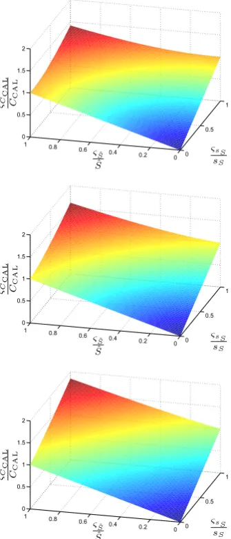
Figure 1 shows the relation of these three relative deviations for different levels of correlation.

0

Figure 1: Error propagation of the relative deviations of the am-plitude (Sˆ) and the width (ss) resulting in the relative deviation

of the calibration constantCCAL. Top: no correlation betweenSˆ

andss. Center:ρ= 0.3. Bottom:ρ= 0.7.

4 DATA SETS

Empirical analysis was carried out on the example of two full-waveform ALS campaigns. The campaigns took place over the Sch¨onbrunn area in Vienna, Austria on August 20, 2004 and May 4, 2005, resp. Both were operated with a Riegl LMS-Q560 instru-ment (Riegl, 2011). The first campaign consisted of eleven flight strips with1.9million to2.9million laser pulses per flight strip and26.4million laser pulses in total. The scanner was operated at a pulse repetition rate of50 kHz.

The second campaign contained thirteen flight strips with3.6 mil-lion to5.0million laser pulses per flight strip, resulting in ap-prox.53.1million laser pulses all together. The pulse repetition rate was100 kHz. The scan layout of both campaigns is shown in Figure 2.

Figure 2: Digital surface model of the Sch¨onbrunn area of Vienna overlaid with the flight trajectories of the two scanning campaigns of 2004 (black lines) and 2005 (blue lines).

The scan layouts of the two campaigns were nearly equivalent with the exception of the different pulse repetition rate and the two additional strips of the 2005 campaign (strips 2 and 14). The two campaigns form therefore an ideal test data set for investigat-ing the validity of the calibration constant among different flight strips and different scanning campaigns regarding the variation of the emitted laser pulses.

5 RESULTS

For each recorded system waveform, its amplitudeSˆand width sswere calculated using the Gaussian Decomposition algorithm

suggested in (Wagner et al., 2006). We based our analysis on his-tograms and other statistics (minimum, maximum, mean, stan-dard deviation and relative stanstan-dard deviation), calculated per flight strip forSˆandss.

The 2004 campaign showed very similar distributions ofSˆ(given in Table 1 and Figure 3) with slightly different mean values per strip but very similar shapes. Only the flight strips 10 and 11 showed a noticeably higher skewness. The distributions ofssper

Flight strip min. max. µ_Sˆ ς_Sˆ ς_Sˆ/µ_Sˆ

1 193.4 264.3 226.0 7.3 0.032

2 190.7 259.4 224.0 7.2 0.032

3 188.3 256.8 222.8 7.1 0.032

4 192.3 257.3 223.5 7.2 0.032

5 192.6 255.7 223.2 7.2 0.032

6 191.6 260.8 224.6 7.3 0.032

7 185.9 260.8 225.5 7.3 0.032

8 192.3 265.7 225.9 7.3 0.032

9 193.8 262.8 226.9 7.4 0.033

10 198.4 265.6 228.7 7.5 0.033

11 199.8 268.1 228.4 7.5 0.033

Mean — — 225.4 7.3 0.032

Table 1: Statistics for the system waveform amplitudesSˆof the 2004 campaign (unit: DN). Bold figures denote the minima and maxima per category for the whole campaign, resp.

200 205 210 215 220 225 230 235 240 245 250 0

0.05 0.1 0.15 0.2 0.25

rel. Frequency

System Waveform Amplitude [DN]

Strip 1 Strip 2 Strip 3 Strip 4 Strip 5 Strip 6 Strip 7 Strip 8 Strip 9 Strip 10 Strip 11

Figure 3: Histogram of the system waveform amplitudesSˆper flight strip in the 2004 campaign (bin size:5).

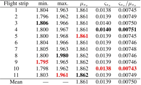
Flight strip min. max. µss ςss ςss/µss

1 1.804 1.963 1.861 0.0138 0.00745 2 1.796 1.962 1.861 0.0139 0.00749 3 1.806 1.966 1.861 0.0140 0.00750 4 1.800 1.967 1.861 0.0140 0.00751

5 1.800 1.968 1.861 0.0139 0.00745 6 1.804 1.966 1.861 0.0139 0.00746 7 1.805 1.963 1.861 0.0139 0.00748 8 1.800 1.980 1.862 0.0139 0.00746

9 1.795 1.965 1.862 0.0139 0.00746

10 1.798 1.962 1.862 0.0138 0.00743 11 1.803 1.961 1.862 0.0139 0.00749

Mean — — 1.861 0.0139 0.00750

Table 2: Statistics for the system waveform widthsssof the 2004

campaign (unit:ns). Bold figures denote the minima and maxima per category for the whole campaign, resp.

1.8 1.85 1.9 1.95

0 0.05

0.1 0.15 0.2 0.25 0.3 0.35 0.4

rel. Frequency

System Waveform Width [ns]

Strip 1 Strip 2 Strip 3 Strip 4 Strip 5 Strip 6 Strip 7 Strip 8 Strip 9 Strip 10 Strip 11

Figure 4: Histogram of the system waveform widthsssper flight

strip in the 2004 campaign (bin size:0.01).

The high similarity of the distributions of bothSˆandssin the

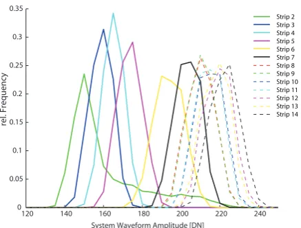
2004 campaign was not present in the other campaign. Especially the amplitudes showed a much higher variation which might be due to the higher pulse repetition rate. The mean values per flight strip ranged from158.8to222.7whereas the average value in the 2004 campaign was225.4. However, the relative deviations per flight strip were comparable to those of the 2004 campaign, ex-cept for strip 2 where the relative deviation was more than three times higher. The two very small minimum amplitudes of strip 11 and 12 (1.2and3.6) are due to a erroneous recording, i.e. the dig-itizer was turned on although no laser pulse was emitted and only noise was recorded. Table 3 and Figure 5 contain the detailed figures and histograms.

Flight strip min. max. µ_Sˆ ς_Sˆ ς_Sˆ/µ_Sˆ

2 126.8 242.8 161.2 19.5 0.121

3 135.4 185.1 158.8 5.7 0.036

4 143.3 189.0 165.1 5.5 0.033

5 148.3 199.6 173.7 6.2 0.036

6 160.9 224.2 193.7 7.5 0.038

7 174.9 232.5 203.3 6.5 0.032

8 179.6 242.3 210.3 7.1 0.034

9 180.4 240.1 210.4 6.9 0.033

10 183.2 244.5 214.9 7.0 0.033

11 3.6 245.6 214.5 6.9 0.032

12 1.2 249.9 219.6 7.1 0.032

13 188.9 247.2 218.3 6.9 0.032

14 188.1 252.8 222.7 7.2 0.032

Mean — — 197.4 7.7 0.040

120 140 160 180 200 220 240 0

0.05 0.1 0.15 0.2 0.25 0.3 0.35

rel. Frequency

System Waveform Amplitude [DN]

Strip 2 Strip 3 Strip 4 Strip 5 Strip 6 Strip 7 Strip 8 Strip 9 Strip 10 Strip 11 Strip 12 Strip 13 Strip 14

Figure 5: Histogram of the system waveform amplitudesSˆper flight strip of the 2005 campaign (bin size:5).

The average of the pulse widthsss in the 2005 campaign

dif-fered about1.5%from the average value of 2004 (1.835 nsvs.

1.861 ns) with lower relative deviations. All flight strips showed

very similar distributions, in contrast to the distributions ofSˆ(see Table 4 and Figure 5).

Flight strip min. max. µss ςss ςss/µss

2 1.775 1.882 1.832 0.00911 0.00497

3 1.777 1.877 1.832 0.00894 0.00488 4 1.767 1.880 1.835 0.00871 0.00475 5 1.775 1.881 1.835 0.00840 0.00458 6 1.783 1.873 1.834 0.00786 0.00428 7 1.777 1.876 1.834 0.00770 0.00420 8 1.781 1.877 1.835 0.00763 0.00416 9 1.786 1.874 1.836 0.00763 0.00416 10 1.774 1.875 1.836 0.00761 0.00414

11 0.363 1.882 1.837 0.00765 0.00416

12 1.776 2.207 1.837 0.00756 0.00410 13 1.776 1.875 1.837 0.00756 0.00412 14 1.782 1.879 1.838 0.00749 0.00408

Mean — — 1.835 0.00800 0.00440

Table 4: Statistics for the system waveform widthsssof the 2005

campaign (unit:ns). Bold figures denote the minima and maxima per category for the whole campaign, resp.

1.8 1.85 1.9 1.95

0 0.05 0.1 0.15 0.2 0.25 0.3 0.35 0.4 0.45 0.5

rel. Frequency

System Waveform Width [ns]

Strip 2 Strip 3 Strip 4 Strip 5 Strip 6 Strip 7 Strip 8 Strip 9 Strip 10 Strip 11 Strip 12 Strip 13 Strip 14

Table 5: Histogram of the system waveform widthsssper flight

strip of the 2005 campaign (bin size:0.01).

Besides the statistics of amplitudes and widths of the emitted laser pulses, also their correlation coefficientsρwere calculated per flight strip. Their values varied from0.23to0.24in the 2004 campaign and from0.02to0.18in the campaign of 2005.

These results enable us to calculate upper bounds of their in-fluence on the calibration constant by evaluating Equation (12). Taking the respective maximal values in Tables 1–4, we see that the relative deviation ofCCALis

ςCCAL

CCAL ≤

p

0.0332_{+ 0.00751}2_{+ 2}

·0.24·0.033·0.00751

= 0.0356

within the single flight strips of 2004,

ςCCAL

CCAL

= p0.1212_{+ 0.00497}2_{+ 2}

·0.14·0.121·0.00497

= 0.1218

for strip 2 of the 2005 campaign (whereρ= 0.14) and

ςCCAL

CCAL ≤

p

0.0382_{+ 0.00488}2_{+ 2}

·0.18·0.038·0.00488

= 0.0392

for all other single strips of this campaign. The variation ofSˆcan be regarded as main influence quantity for the variation ofCCAL

so thatssand the correlation between these two parameters can

be neglected.

Our results also apply if an other deconvolution technique than Gaussian Decomposition is performed. In this case, the right-hand side of Equation (6) is taken into account so that the relative deviation ofCCALis only dependent on the relative deviation of

system waveform energy,ςES/ES. Their distribution was also

analysed but not separately listed here. It showed a distribution similar to the one of the system waveforms’ amplitudes as was expected due to the small variations of the widthsss.

6 DISCUSSION AND OUTLOOK

In this study, the variations of emitted laser pulses were evalu-ated on behalf of two flight campaigns of 2004 and 2005, one operated with a pulse repetition rate of50kHz, the other with

100kHz. The results of the 2004 campaign showed similar dis-tributions for all flight strips whereas the 2005 data set is charac-terized by narrow distributions within the single flight strips but significantly different behaviour between this strips. The relative deviation ofCCALwas around3−4%per flight strip in our data

sets. However, it was a lot higher within the whole 2005 ALS campaign as well as between the 2004 and the 2005 campaign although the same instrument was in use. The mean value for the system waveform amplitudes amounted to225.4with a relative deviation of3.2%in the 2004 campaign and to197.4in the 2005 campaign (relative deviation: 4.0%). The mean of the system waveform widths resulted to1.861 nsand1.835 ns, resp. In both cases, their relative deviations were smaller than1%.

of an individual calibration constant per strip. This would allow to reduce the variation of the radiometric calibration between the strips. The determination of a shot-based calibration constant is not feasible. However, in order to consider the individual varia-tion of the laser pulse, either

• the individual amplitudes and pulse widths can be consid-ered as additional variables in the whole radiometric cali-bration process (cf. (Wagner, 2010)) or

• by using echo parameters normalized by the parameters of the individual laser pulses instead of the original echo pa-rameters in the mathematical framework of radiometric cal-ibration. This would enable to consider the pulse variations without increasing storage space and processing time. Fur-thermore, it is compatible with currently available file for-mat standards.

Future research and further practical investigations will show which of these methods is more practicable.

ACKNOWLEDGEMENTS

We would like to thank Schloß Sch¨onbrunn Kultur- und Betrieb-sges.m.b.H and Milan-Flug GmbH for their support in the data acquisition campaigns. Furthermore, we want to thank Norbert Pfeifer and Helmut Kager (both IPF) for the fruitful discussions.

The first author has been supported by a Karl Neumaier PhD scholarship.

The Ludwig Boltzmann Institute for Archaeological Prospection and Virtual Archaeology is based on an international coopera-tion of the Ludwig Boltzmann Gesellschaft (Austria), the Uni-versity of Vienna (Austria), the Vienna UniUni-versity of Technol-ogy (Austria), the Austrian Central Institute for MeteorolTechnol-ogy and Geodynamics, the office of the provincial government of Lower Austria, RGZM (Roman-Germanic Central Museum Mainz, Ger-many), RA (Swedish National Heritage Board), VISTA (Visual and Spatial Technology Centre, University of Birmingham, UK) and NIKU (Norwegian Institute for Cultural Heritage Research).

References

ASPRS, 2011. LAS file format exchange activ-ities. http://www.asprs.org/Standards/ LASer-LAS-File-Format-Exchange-Activities. html. Homepage of ASPRS LAS file format, accessed: April 2011.

Bretar, F., Chauve, A., Bailly, J.-S., Mallet, C. and Jacome, A., 2009. Terrain surfaces and 3-d landcover classifica-tion from small footprint full-waveform lidar data: Ap-plication to badlands. Hydrology and Earth System Sci-ences 13(8), pp. 1531–1545.

Briese, C., H¨ofle, B., Lehner, H., Wagner, W. and Pfenning-bauer, M., 2008. Calibration of full-waveform airborne laser scanning data for object classification. In: SPIE: Laser Radar Technology and Applications XIII.

H¨ofle, B. and Pfeifer, N., 2007. Correction of laser scan-ning intensity data: Data and model-driven approaches. ISPRS Journal of Photogrammetry and Remote Sensing 62(6), pp. 415–433.

Hofton, M., Minster, J. and Blair, J., 2000. Decomposi-tion of laser altimeter waveforms. IEEE TransacDecomposi-tions on Geoscience and Remote Sensing 38, pp. 1989–1996.

Jelalian, A. V., 1992. Laser Radar Systems. Artech House, Boston.

Jutzi, B. and Stilla, U., 2006. Range determination with waveform recording laser systems using a wiener filter. ISPRS Journal of Photogrammetry and Remote Sensing 61(1), pp. 95–107.

Kaasalainen, S., Hyypp¨a, H., Kukko, A., Litkey, P., Ahokas, E., Hyypp¨a, J., Lehner, H., Jaakkola, A., Suomalainen, J., Akujarvi, A., Kaasalainen, M. and Pyysalo, U., 2009. Radiometric calibration of lidar intensity with commer-cially available reference targets. IEEE Transactions on Geoscience and Remote Sensing 47(2), pp. 588–598.

Lehner, H. and Briese, C., 2010. Radiometric calibration of full-waveform airborne laser scanning data based on natural surfaces. In: ISPRS Technical Commission VII Symposium 2010: 100 Years ISPRS – Advancing Remote Sensing Science. International Archives of the Photogrammetry, Remote Sensing and Spatial Informa-tion Sciences 38 (Part 7B), Vienna, Austria, pp. 360– 365.

Mallet, C., 2011. Analyse de donn´ees lidar `a Retour d’Onde Compl`ete pour la classification en milieu ur-bain. PhD thesis, T´el´ecom ParisTech, ´Ecole Doctorale d’Informatique, T´el´ecommunications et ´Electronique de Paris, Paris, France.

Mallet, C. and Bretar, F., 2009. Full-waveform topographic lidar: State-of-the-art. ISPRS Journal of Photogramme-try and Remote Sensing 64(1), pp. 1–16.

Mikhail, E. M., 1976. Observations And Least Squares. IEP-A Dun-Donnelley, New York.

Parrish, C. E. and Nowak, R. D., 2009. Improved Ap-proach to Lidar Airport Obstruction Surveying Using Full-Waveform Data. Journal of Engineering Surveying 135(2), pp. 72–82.

Riegl, 2011.www.riegl.com. Homepage of the company RIEGL Laser Measurement Systems GmbH, accessed: April 2011.

Roncat, A., Bergauer, G. and Pfeifer, N., 2011. B-Spline Deconvolution for Differential Target Cross-Section Determination in Full-Waveform Laser Scanner Data. ISPRS Journal of Photogrammetry and Remote Sens-ing 66(4), pp. 418–428.

Wagner, W., 2010. Radiometric calibration of small-footprint full-waveform airborne laser scanner measure-ments: Basic physical concepts. ISPRS Journal of Pho-togrammetry and Remote Sensing 65(6 (ISPRS Cente-nary Celebration Issue )), pp. 505–513.