1. INTRODUCTION
Since the term of "Big Data" presented by NASA scientists in 1997 (Cox and Ellsworth 1997), the meaning or definition of big data has seemed to be another 'big data' as stated by Press (Press 2014). In general, big data implies massive data that challenge traditional processing techniques. The analysis of big data is related with the process of exploring huge data which can be structured or unstructured to unearth hidden patterns and correlations that conventional approach cannot find out (Erl 2016). Three major characteristics of big data are volume, velocity and variety (Hilbert 2016; Laney 2001). Landsat imagery (USGS 2015) satisfies these characteristics because of massive data archive since 1972, continuous temporal updates, and various spatial resolutions from different sensors.
Since the Landsat scenes were available to the public, free of charge on December 18, 2008, Landsat imagery has been used for various applications such as landuse/landcover change, software development, education, climate science, agriculture, ecosystem monitoring, forestry, water and fire, to name a few. However, attention was seldom given to Landsat big data analysis. Considering the paradigm shifting role of big data analysis in Geography and other fields (Wyly 2014), the vast archive and long-term time-series Landsat big data opens new opportunities for researchers to explore new methodologies and findings in remote sensing and geospatial analyses.
This research focuses on analyzing reflectance changes on water surfaces. While many remote sensing research projects have been performed with long-term MODIS, AVHRR and Landsat datasets, their focuses have mostly been on plant phenology, urban dynamics and large ocean water bodies. Little attention has been given on the long-term water quality analysis using Landsat imagery.
The Han River (a.k.a. "HanGang") in South Korea was analyzed in this research. The Han River watershed has experienced dramatic land cover change over the last some decades. Particularly, multiple algal blooms have been reported in 2015. Various research projects have been carried out about the Han River. Some examples are the simulation of water quality with pollution sources (Lee and Kim 2008), algal characteristics analyses (Kim et al. 1998), the big data mapping of algal amounts measured at water quality monitoring stations (Seoul City 2015), and modeling algal amounts in association with field measurements (Suh et al. 2006). None of these research projects, however, tackled the analysis of long-term Landsat time-series analysis.
Considering the significance of examining the Han River water quality over a long term period, this research aims at identifying locational variance of reflectance, analyzing seasonal difference, finding long-term trend, and modeling algal amount variation using Landsat big data.
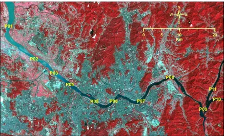
2. STUDY AREA, DATA AND METHODOLOGIES Figure 1 shows the Han River, Seoul and vicinity. The yellow labels indicate eleven sampling points along the river. The river flows from the right-hand side (east) to the left (west), into the Yellow Sea. In the figure, the upstream (i.e. P09 – P11) are much darker than the downstream (i.e. P01 and P02). There are two overflow dams. One is the ShinGok overflow dam between P02 and P03, and the other is JamSilDaeGyo near to P07. One major dam (a.k.a. PalDang Dam) is located below P09, creating a large reservoir to supply water for metropolitan Seoul.
LANDSAT BIG DATA ANALYSIS FOR DETECTING LONG-TERM WATER QUALITY
CHANGES: A CASE STUDY IN THE HAN RIVER, SOUTH KOREA
J. C. Seonga,*, C. S. Hwangb, R. Gibbsa, K. Roha, M. R. Mehdic, C. Ohd, J. J. Jeonge
a Dept. of Geosciences, University of West Georgia, Carrollton, Georgia, USA –
([email protected], [email protected], [email protected])
b Dept. of Geography, Kyunghee University, Seoul, South Korea - [email protected] c NED University of Engineering & Technology, Karachi, Pakistan - [email protected] d Dept. of GIS Engineering, NamSeoul University, CheonAn, South Korea - [email protected] e Dept. of Geography, SungShin Women's University, Seoul, South Korea - [email protected]
KEYWORDS: Big data, Landsat, Han River, reflectance, water quality, remote sensing
ABSTRACT:
Landsat imagery satisfies the characteristics of big data because of its massive data archive since 1972, continuous temporal updates, and various spatial resolutions from different sensors. As a case study of Landsat big data analysis, a total of 776 Landsat scenes were analyzed that cover a part of the Han River in South Korea. A total of eleven sample datasets was taken at the upstream, mid-stream and downmid-stream along the Han River. This research aimed at analyzing locational variance of reflectance, analyzing seasonal difference, finding long-term changes, and modeling algal amount change. There were distinctive reflectance differences among the downstream, mid-stream and upstream areas. Red, green, blue and near-infrared reflectance values decreased significantly toward the upstream. Results also showed that reflectance values are significantly associated with the seasonal factor. In the case of long-term trends, reflectance values have slightly increased in the downstream, while decreased slightly in the mid-stream and upstream. The modeling of chlorophyll-a and Secchi disk depth imply that water clarity has decreased over time while chlorophyll-a amounts have decreased. The decreasing water clarity seems to be attributed to other reasons than chlorophyll-a.
Seoul and vicinity where Han River flows through are covered by one Landsat scene (World Reference System -2 Path 116 and Row 034). A total of 776 scenes (May 10, 1984 ~ November 17, 2015) were downloaded from the U.S. Geological Survey website (http://EarthExplorer.USGS.gov). The Landsat Surface Reflectance High Level Data Products were downloaded in this research for data consistence among different sensors (i.e. TM, ETM+ and OLI) and for simplification of data processing. The reflectance datasets also resolved the different quantization issues between OLI and the other sensors. The Bulk Download tool in the EarthExplorer did not work with the reflectance datasets, so the ESPA Bulk Download Client (http://landsat.usgs.gov/CDR_LSR.php) was used.
Downloaded files were in the *.tar.gz format. The ESTsoftTM
Alzip tool (http://www.altools.com) was used to uncompress the *.gz files to make *.tar files. The Alzip tool was very useful because it supported the command-line user interface with a batch file.
Each tar file contains many bands and additional files. The blue, green, red, near infrared and CFmask layers were extracted using the Alzip tool. Extracted files were renamed and grouped into five folders – Blue, Green, Red, near infrared (NIR) and CFmask. With each folder containing 776 TIF files, QGIS version 2.12 (http://www.qgis.org) was used to create five VRT files, i.e. one for each folder (QGIS Raster Miscellaneous Build Virtual Raster). During the creation of VRT files, the "Source No Data" option was checked and set to 0. The "Separate" option was checked too. The "Load into canvas when finished" option was unchecked due to an error when it was checked.
The pixel values at the eleven sampling locations (i.e. P01 ~ P11 in Figure 1) were identified using the Value Tool plugin in QGIS. Table 1 shows the sampling locations.
Point x-coordinate y-coordinate P01 294,600.65 4,176,086.56
P02 301,702.39 4,166,854.61
P03 307,312.97 4,162,882.64
P04 311,794.92 4,159,663.62
P05 318,690.80 4,154,894.15
P06 324,060.01 4,154,942.31
P07 331,740.20 4,154,971.22
P08 339,894.16 4,161,651.61
P09 349,193.05 4,152,683.60
P10 353,051.82 4,155,466.64
P11 351,884.81 4,158,342.54
Table 1. Sample point locations (Unit: meters in UGS84 UTM zone 52N)
The identified pixel values were re-arranged and filtered in Excel. First of all, the CFmask layer was used to filter cloud-free pixels. The CFmask layer contains six number flags indicating Fill (255), Clear (0), Water (1), Shadow (2), Snow (3) and Cloud (4). The datasets with the Clear or Water flags were used in this research. The surface reflectance values beyond the valid range (0 ~ 10000 with the scale factor of 0.0001) were removed too. There were one or two cases of reflectance values larger than 10000 in each sample point and they were mostly from L7 and occasionally from L5. There were two cases of abnormal outliers (3000 or larger in reflectance) and they were removed too with a consideration that the spectral reflectance from water is mostly less than 30%. After data cleanup, about Figure 1. The Han River, Seoul and vicinity. This Landsat 8 imagery was composited using the
31% of original datasets were identified as 'clean' and they were used for further analyses. Finally, the Excel worksheets were converted to comma-separated value (CSV) files and they were imported into the R package for further statistical analyses.
3. RESULTS
3.1 Change of Reflectance along the Han River
Figure 2 shows the boxplots of the reflectance values of the blue, green, red and infrared bands at the sample points 01 through 11. In the case of the blue, green and red bands, three distinctive groups are apparent. The first group (Group 01) is P01 and P02 at the downstream that are located below the ShinGok overflow dam. The second group (Group 02) is
composed of P03 through P08 that are located between the ShinGok overflow dam and the PalDang Dam. The last group (Group 03) consists of P09 through P11 at the upstream that are located above the PalDang Dam.
Reflectance values in the blue, green and red bands decrease significantly toward the upstream as shown in Table 2. The table also shows that the reflectance values are distinctively different among three sampling location groups in the blue, green and red bands. In the case of the near infrared band, Group 02 and Group 03 sample points are not significantly different as shown by the TukeyHSD analysis (p-value = 0.229). The ANOVA F statistic values also indicate that the largest difference among groups appears in the red band, followed by green, blue and NIR bands.
Table 2. ANOVA analyses of reflectance values among different sample locations
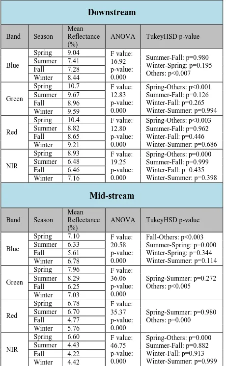
3.2. Seasonal change of reflectance values
In order to analyze the seasonal change of reflectance values, significant locational factor that was identified in Section 3.1.
Downstream
Table 3. Effect of seasonal factor on band reflectance
The effect of seasonal factor on band reflectance is summarized in Table 3. The low p-values of the ANOVA analysis results Spring and summer reflectances are similar in the green and red bands. NIR reflectances are particularly high during the spring season. In the downstream, spring reflectances are significantly high in the four bands and summer and fall are similar in most bands.
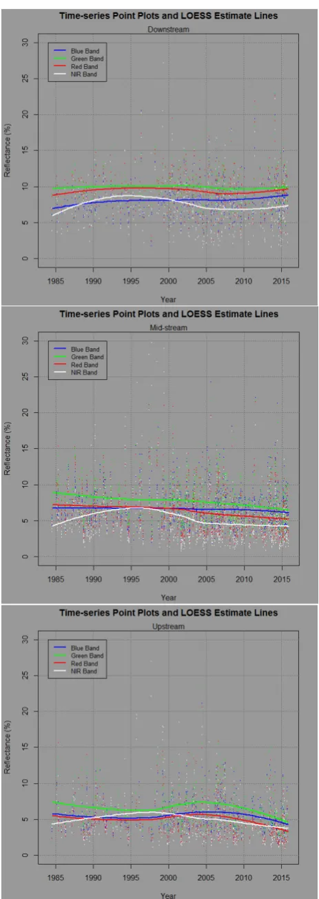
3.3. Time-series change of reflectance values
The time-series changes of reflectance values were analyzed in the Downstream, Mid-stream and Upstream. Figure 3 shows how the reflectance values have changed since 1984. In the figures, each point indicates a reflectance value at a sample point in a Landsat scene. Since there are multiple sample points in a scene and four bands (i.e. Blue, Green, Red and NIR bands) are plotted, multiple points appear virtically lined up in the band reflectance values are rather constant. A significant increase of near-infrared reflectance values appears during the 1990s. In the case of the Upstream area, 2~3% decreases appear in the red, green and blue bands with short-term increases around 2005. In the case of the NIR band, it shows an increase untill the late 1990s, but decrease during the 2000s.
The R2 values of the LOESS models in Table 4 are low because
of the large amounts of residuals. Overall, the R2 values
increase significantly towards the Upstream. The highest R2
Figure 3. Temporal change of reflectance values at the Downstream, Mid-stream and Upstream areas
Table 4. R2 values of the LOESS models shown in Figure 3
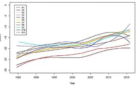
3.4. Modeling Chlorophyll-a Amounts and Secchi Depths Many chlorophill or Secchi disk depth estimation models have been developed using Landsat imagery (e.g. Brezonik et al. 2005; Moreno 2013; Hellweger et al. 2004; Han and Jordan 2005; Vincent et al. 2004; Krizanich and Finn 2009; Trescott 2012; Hoyer et al. 2002). In this research, Trescott's models (Trescott 2012, p.40 & p.45) were used to estimate the trends of Chlorophyll-a (Chl-a) and Secchi depth (SD) changes over time because they were derived by field measurements from mid-latitude fresh water bodies:
Chl-a (μg/L) = -46.51 + 105.30 (B2/B1) – 40.39(B3/B1) (1)
SD(m) = 26.07 – 23.26 (B2/B1) – 17.19 (B3/B1) (2)
B1, B2 and B3 are the blue, green and red band reflectance values, respectively. In this research, the estimated values with the LOESS models in Section 3.3 were used with Equations (1) and (2). Figure 4 and Figure 5 show the changes of estimated amounts. In general, the models show decreasing trends of chlorophyll-a amounts and Secchi disk depth. In the case of sample points P05 and P11, increasing amounts of chlorophyll-a chlorophyll-appechlorophyll-ar chlorophyll-after 2010 chlorophyll-and the Secchi disk depths increchlorophyll-ase too.
Considering that decreasing chlorophyll amounts increase Secchi disk depth in general, the opposite results shown in Figures 4 and 5 seem be attributed to (1) the dissolved organic substances or compounds that change water color, (2) non-algal particulates such as clay or sand, or (3) aquatic macrophytes like water plants (For more information, refer to Florida LAKEWATCH 2001).
Figure 4. Temporal change of the estimated chlorophyll-a amount at the eleven sample points
Figure 5. Temporal change of the estimated Secchi disk depth (m) at the eleven sample points
4. CONCLUSIONS
This research has demonstrated how long-term Landsat big data can be used for investigating freshwater quality and the changes over a long time period. A total of 776 Landsat scenes were analyzed in this research to identify the locational variance of reflectance along the Han River, its seasonal differences and the long-term trend. The temporal changes in chlorophyll-a and Secchi disk depth were also examined to estimate algal amount variation.
The results showed that there were distinctive reflectance differences among the downstream, mid-stream and upstream of the Han River. The red, green, blue and near-infrared values decreased significantly toward the upstream. It was also found that the reflectance values were significantly associated with seasons. In the downstream, most of the bands exhibited much higher reflectance values in spring than in other seasons, while there were relatively little differences between summer and fall. In the mid-stream, spring and summer reflectance values were similar in the green and red bands but not in the blue and NIR bands. In the case of the upstream, the reflectance values in the green and red bands were lower in fall compared to the rest of the year and a similar difference was found in the NIR band for spring.
The long-term time series trends in Section 3.3 indicate that the red, green, blue and NIR reflectance values have slightly increased in the downstream of the Han River, while they have decreased in the mid-stream and upstream. The modeling of chlorophyll-a and Secchi disk depth in Section 3.4 implies that water clarity has decreased over the years, and chlorophyll-a amounts have also decreased. The decreasing water clarity seems to be attributed to other reasons than chlorophyll-a such as dissolved organic substances or compounds that change water color and non-algal particulates like clay or sand. Further research may reveal the reason for decreasing water clarity more clearly.
ACKNOWLEDGMENTS
The project described in this publication was supported by Grant Number G14AP00002 from the Department of the Interior, United States Geological Survey to AmericaView (http://www.AmericaView.org). Its contents are solely the responsibility of the authors; the views and conclusions contained in this document are those of the authors and should not be interpreted as representing the opinions or policies of the
U.S. Government. Mention of trade names or commercial products does not constitute their endorsement by the U.S. Government.
REFERENCES
Brezonik P., Menken, K.D. and Bauer, M., 2005. Landsat-based remote sensing of lake water quality characteristics, including chlorophyll and colored dissolved organic matter. Lake and Reservoir Management 21(4): 373-382.
Cox, M. and Ellsworth, D., 1997. Application-controlled demand paging for out-of-core visualization, VIS '97 Proceedings of the 8th conference on Visualization '97, pp.235-244. IEEE Computer Society Press, Los Alamitos, CA, USA.
Erl, T., Khattak, W., and Buhler, P., 2016, Big Data Fundamentals: Concepts, Drivers & Techniques, Prentice Hall.
Laney, D., 2001, 3D Data Management: Controlling Data Volume, Velocity and Variety. In "Application Delivery Strategies," by META Group. http://blogs.gartner.com/doug- laney/files/2012/02/ad1074-The-Great-Enterprise-Balancing-chlorophyll-a concentration in Pensacola Bay, Florida using Landsat ETM+ data. International Journal of Remote Sensing 26(23): 5245–5254.
Hancock, M.J., 2015. Predicting water quality by relating Secchi disk transparency depths to Landsat 8. Masters Thesis. Department of Geography, Indiana University.
Hellweger, F.L., Schlosser, P., Lall, U., Weissel, J.K., 2004. Use of satellite imagery for water quality studies in New York Harbor. Estuarine, Coastal and Shelf Science 61: 437–448.
Hilbert, M., 2016. Big Data for Development: A Review of Promises and Challenges. Development Policy Review, 34(1), 135–174. http://doi.org/10.1111/dpr.12142.
Hoyer, M.V., Frazer, T.K., Notestein, S.K. and Canfield, D.E. Jr., 2002. Nutrient, chlorophyll, and water clarity relationships in Florida’s nearshore coastal waters with comparisons to freshwater lakes. Canadian Journal of Fisheries and Aquatic Sciences 59: 1024–1031.
Kim, Y.J., Kim, M.W. and Kim, S.J., 1998. Ecological Characteristics of Phytoplankton Community in the Mid- and Downstream of the Han River. Algae 13(3): 331-338.
Krizanich, G.W. and Finn, M.P., 2009. Table Rock Lake Water-Clarity Assessment Using Landsat Thematic Mapper Satellite Data. U.S. Geological Survey, Scientific Investigations Report 2009–5162, 9p.
Lee, C.Y. and Kim, K.H., 2008. Development of GIS based Water Quality Simulation System for Han River and Kyeonggi Bay Area. Journal of Korea Spatial Information Society 10 (4): 77-88.
Press, G., 2014. 12 Big Data Definitions: What's Yours?, Forbes news article (September 3, 2014). URL: http://www.forbes.com /sites/gilpress/2014/09/03/12-big-data-definitions-whats-yours/#75d75d9121a9
Seoul City, 2015. Algal Map. URL: http://m.arisu.seoul.go.kr /_sudo_news/report_detail.jsp?nID=327.
Suh, M.Y., Gil, H.K., Kim, K.S., Jeong, H.J., Kim, J.Y., Yoon, J.C., Lim, G.C., Lee, J.H., Lee, S.C., Kim, H.S., Bae, K.S. and Eom, S.W., 2006. Fluctuation of Environmental Factors & Dynamics of Phytoplankton Community in the Han River. Report of Seoul Research Institute of Public Health & Env. 42:453~464. URL: https://opengov.seoul.go.kr/research/6410377
Trescott, A., 2012. Remote Sensing Models of Algal Blooms and Cyanobacteria in Lake Champlain. Masters Thesis, Univ. of Massachusetts–Amherst. URL: http://scholarworks.umass.edu /cee_ewre/48.
USGS (US Geological Survey), 2015, Landsat 8 (L8) Data Users Handbook. URL: https://landsat.usgs.gov/documents /Landsat8DataUsersHandbook.pdf
Vincent, R.K., Qin, X, McKay, M.L., Miner, J., Czajkowski, K., Savino, J. andBridgeman, T., 2004. Phycocyanin detection from LANDSAT TM data for mapping cyanobacterial blooms in Lake Erie. Remote Sensing of Environment 89: 381– 392.